Rapidly-Exploring Random Tree

A Rapidly-Exploring Random Tree (RRT) is a fundamental path planning algorithm in robotics, first developed by Steven LaValle in 1998 (see References). Path planning is the task of moving a robot from one location to another, while avoiding obstacles and satisfying constraints.

An RRT consists of a set of vertices, which represent configurations in some domain \(D\) and edges, which connect two vertices. The algorithm randomly builds a tree in such a way that, as the number of vertices \(n\) increases to \(\infty\), the vertices are uniformly distributed across the domain \(D \subset \mathbb{R}^n\).

The algorithm, as presented below, has been simplified from the original version by assuming a robot with dynamics \(\dot{q} = u\) where \(\lVert u \rVert = 1\) and assuming that we integrate the robot's position forward for \(\Delta t = 1\). These simplifications are described and removed in Task 4.

Some pseudocode for the simplified algorithm is as follows:

RRT Algorithm
  Input:
      \(q_{\text{init}} \leftarrow \text{Initial configuration} \)
      \(K \leftarrow \text{Number of vertices in RRT}\)
      \(\Delta \leftarrow \text{Incremental distance}\)
      \(D \leftarrow \text{The planning domain}\)
  Output:
      \(G \leftarrow \text{the RRT}\)

  Initialize \(G\) with \(q_\text{init}\)
  repeat \(K\) times
    \(q_\text{rand}\) ← RANDOM_CONFIGURATION(\(D\))
    \(q_\text{near}\) ← NEAREST_VERTEX(\(q_\text{rand}\), \(G\))
    \(q_\text{new}\) ← NEW_CONFIGURATION(\(q_\text{near}\), \(q_\text{rand}\), \(\Delta\))
    Add vertex \(q_\text{new}\) to \(G\)
    Add an edge between \(q_\text{near}\) and \(q_\text{new}\) in \(G\)
  end repeat
  return \(G\)

• RANDOM_CONFIGURATION Generates a random position in the domain.
• NEAREST_VERTEX finds the vertex in \(G\) that is closest to the given position, according to some metric (a measure of distance). We will use the Euclidean metric.
• NEW_CONFIGURATION generates a new configuration in the tree by moving some distance \(\Delta\) from one vertex configuration towards another configuration.

The three tasks below are listed in order of increasing difficulty. They each build upon the previous task. The references and notes section at the end has some useful resources.

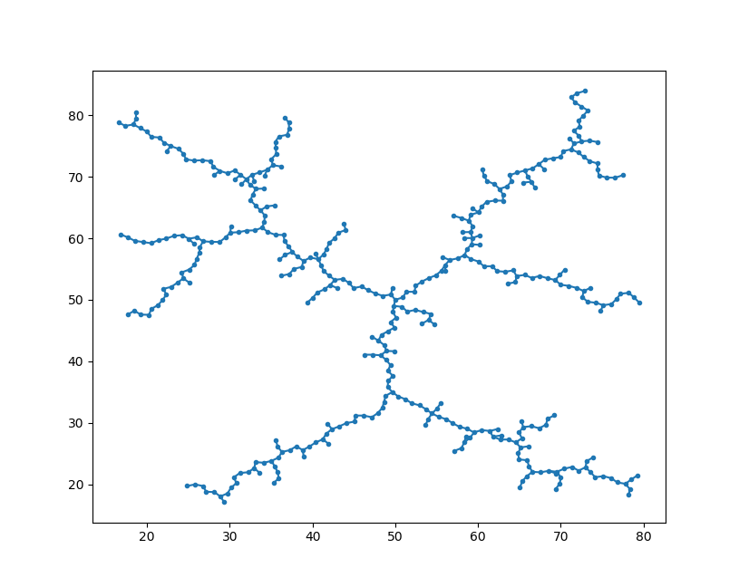
Implement an RRT in a two-dimensional domain, \(D = [0, 100] \times [0, 100]\). Use an initial configuration of \(q_\text{init} = (50, 50)\) and \(\Delta = 1\).

Plot your result for a few different values of \(K\). It should look something like the below image, but of course it will be slightly different due to the randomness.

If you run your program for several thousand iterations, you should see uniform coverage over the whole space.

We will now add circular obstacles to the domain.

There are three modifications to make.

1. Collision Checking: before adding \(q_\text{new}\) to the tree, you must check if the path from \(q_\text{near}\) to \(q_\text{new}\) intersects with an obstacle. If it does not collide, you can add the new vertex and continue the algorithm.
   • A collision occurs if the line between the two vertices intersects any of the obstacle circles.
   • Ignoring vertexes that are in collision is a simplification but adds inefficiency (and is due to our assumption that \(\lVert u \rVert = 1\). If you were to assume that \(\lVert u \rVert \leq 1\), then a vertex could be added along the line from \(q_\mathrm{near}\) to \(q_\mathrm{new}\) such that it is as far as possible from \(q_\mathrm{near}\) without colliding with an obstacle.
2. After adding a new vertex to the tree, you should check for a collision free path from that vertex to the goal. If this exists, you can terminate the algorithm.
3. Once you find a path from a node in the tree to the goal state, you can traverse the tree backwards to the starting location to find the path.
   • You may wish to still count the number of iterations and terminate if a path isn't found in enough iterations.
   • You can terminate the algorithm if a path isn't found after a certain number of iterations.
4. Start by hard-coding a few circles with different radii and get everything working.
5. Start randomizing start locations, goal locations, and obstacle size and locations. Run your code many times to make sure it works.
6. If the start or goal is inside an obstacle, regenerate it.
7. You may wish to create a class that manages the obstacles and collision detection.
8. You may wish to create some unit tests for your code, using non-random starting conditions.
   • See Unit Test for details.
   • The Basic example is enough to get started.
   • While testing your code with random configurations, if you encounter a bug, it may make sense to create a unittest for that case.

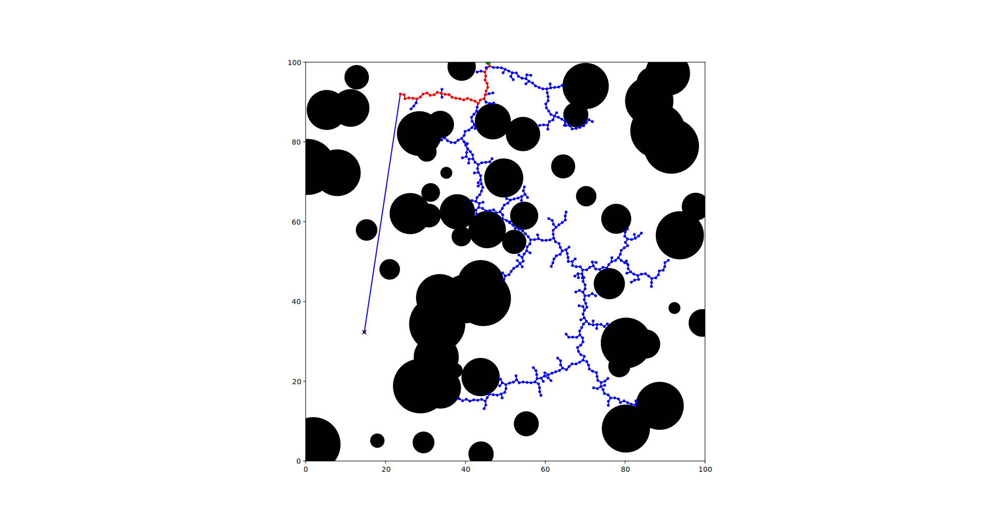
Your code should be able to generate a plot (using matplotlib) with the following output:

1. The circles representing the collision
2. The full RRT
3. The start and end states should be clearly identified
4. The path from start to goal should be indicated

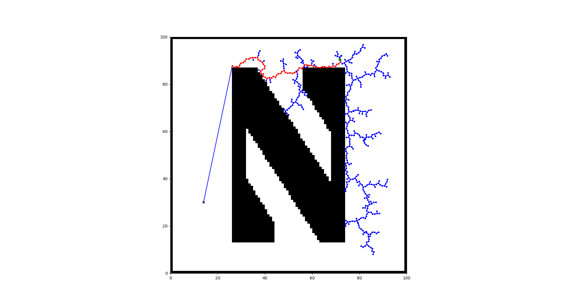
Now let's consider arbitrary objects, represented by black pixels in a binary image.

You should load a binary image into your script, choose starting and goal locations, and then plan a path.

To start, use the image below, start at (40, 40) and end at (60, 60). Collisions occur when the pixel is black. Plot the image in the background of your results

• Aside from the collision detection algorithm, this task is not all that different from the previous one.
• If you used a class for Task 2, you should be able to create a class with the same interface but a different implementation.
• As a challenge, make it easy for a user to plan a path with circular obstacles or from an image, while duplicating as little code as possible.
• A good design would have a simple check for obstacles or images at the beginning and then the rest of the code would be exactly the same for both cases.

The main simplifications made in the above algorithms is to move a by a fixed step-size to find \(q_\mathrm{new}\) and only add that node if it is collision free. This method does not account for the robot dynamics and is inefficient because some iterations of the algorithm do not result in adding a new node to the tree. To account for these differences the algorithm should be modified as follows:

1. NEW_CONFIGURATION should be divided into two steps: SELECT_INPUT and NEW_STATE
   • \(u\) ← \(\text{SELECT_INPUT}(q_\text{rand}, q_\text{near})\) computes a control u that will drive the robot as close to \(q_\text{rand}\) as possible from \(q_\text{near}\) without colliding.
   • \(q_\mathrm{new} = \text{NEW_STATE}(q_\text{near}, u, \Delta t)\) computes the new state if the control \(u\) is applied for \(\Delta t\).
2. Perhaps the simplest robot dynamics to use are \(\dot{q} = u\), with the assumption that \(\lVert u \rVert < 1\).
   • By setting \(\Delta t = 1\) and \(\lVert u \rVert = 1\) we end up with the simplified algorithm above.

Here are some libraries you should use

• matplotlib - for plotting
• numpy - for the math
• imageio - for reading the image

1. The Matplotlib Documentation will be useful
2. There are many ways to plot an RRT.
   • The simplest conceptually is to plot each vertex as a point and plot each edge as a line segment between two connected points.
   • LineCollection can be used to plot the lines. You draw a line collection on an axis ax using ax.add_collection See: LineCollection Example
3. It is often useful to seed the random number generator when testing, which causes it to return the same sequence of numbers every time you run your program.
   • If you use the numpy random number generator, you can seed it with numpy.random.seed.
4. For plotting, it may be helpful to manually set the x and y limits to fit the domain.
5. For collision checking between a circle and a line:
   1. Find the shortest distance between the line-segment (from the RRT) and the circle's center. If this distance is less than the circle's radius there is a collison.
   2. Finding shortest distance between a point and a line may be useful, but leaves some corner cases (due to the distinction between a line and a line segment).
   3. Drawing the situation may help you discover these edge cases.
   4. One approach to this problem is to use a parametric equation of the line. This equation can be written in terms of the end points of a line segment and the value of the parameter determines whether the point is on the line segment.
6. Collision checking in the image obstacles requires checking every pixel along the line segment between the two configurations.
   • The set of all pixels that a line segment overlaps is called the supercover of the line segment.
   • A Fast Voxel Traversal Algorithm for Ray Tracing is one way to ensure that all pixels that intersect with the line are visited.
7. The imread function from the imageio library can be used to load the image.
   • The image is a numpy array of pixels.
   • The pixel coordinate system increases from top to bottom. You can use numpy.flipud to compensate.
   • To show the image, use imshow and, if you flipped it, use origin = 'lower'.
   • You should set cmap = 'gray' to view the image in black and white, since the image is a grayscale image.
   • When accessing an image as an array, rows correspond to y values and columns to x values.
8. To plot the circles, use matplotlib.patches.Circle.

1. The Original RRT Paper by Steven M. LaValle
2. Planning Algorithms by Steven M. Lavalle