RRT Programming Challenge
Table of Contents
1 Introduction
A Rapidly-Exploring Random Tree (RRT) is one of the most important tools used in robotic path planning. RRTs were first developed in 1998 by Steve LaValle at Iowa State. Dr. Lavalle has been a professor at UIUC and University of Oulu, he acted as Chief Scientist of VR/AR/MR for Huawei Technologies, and was one of the inventors of the Oculus Rift. In the simplest of terms, an RRT is an algorithm that guarantees rapid exploration of some vector space. In fact given some domain \({D} \subset \mathbb{R}^n\) it is guaranteed that as the number of vertices in the RRT increases to \(\infty\) the RRT converges on a uniform distribution over all of \(D\).
Generally speaking an RRT is represented in software as a list of vertices contained in the search domain i.e. each vertex \(v \in D\), and a list of edges connecting the vertices. The general algorithm for building an RRT is as follows:
Algorithm
Input: Initial configuration \(q_{init}\), number of vertices in RRT \(K\), incremental distance \(\Delta q\)
Output: RRT graph \(G\)
\(G\).init(\(q_{init}\))
for \(k = 1\) to \(K\)
\(q_{rand}\) ← RAND_CONF()
\(q_{near}\) ← NEAREST_VERTEX(\(q_{rand}\), \(G\))
\(q_{new}\) ← NEW_CONF(\(q_{near}\), \(q_{rand}\), \(\Delta q\))
\(G\).add_vertex(\(q_{new}\))
\(G\).add_edge(\(q_{near}\), \(q_{new}\))
return \(G\)
2 Goals
Below are several goals of increasing complexity related to RRTs. While working on accomplishing these goals, this would be a great time to practice your Git usage. By the time you are done you should have a Git repository with multiple commits. It would be even better if this repo has a remote that you push to and fetch from. If you work with a partner, this would even be a great chance to practice fetching and merging as a means of sharing.
These will likely be challenging tasks. At the bottom of this page, you'll find a few helpful resources to guide you along the way.
2.1 Generate a simple RRT
Consider a domain \(D = [0,100]\times[0,100]\), an initial configuration \(q_{init} = (50,50)\), and a stepsize \(\Delta q = 1\). Use the Euclidean metric for evaluating distance. Write a Python script that constructs and plots an RRT using these conditions. You should be producing plots that look something like the image below.
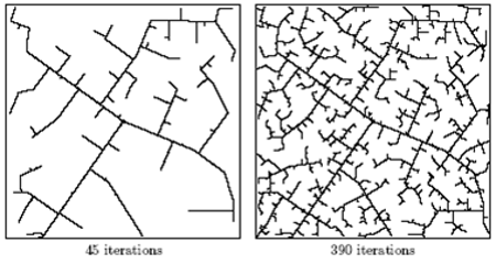
Figure 1: Visualization of an RRT graph borrowed from here.
2.2 RRT path planning with circular collision objects
In this goal you are going to modify the RRT from the previous example to actually accomplish some path planning. For the starting location let's start with \(q_{init} = (10,10)\) and a goal location of \(q_{goal} = (75,75)\). For the representation of our environment, we are going to assume all things we can collide with are easily represented as circular. This way, our collision checking can be performed analytically. To determine if a particular pair of vertices has a safe, collision-free path between them, all we need to do is determine if the line connecting the nodes has an intersection with any of the circles.
So now, the algorithm from the previous section will only add nodes to the tree if they have a collision free path to the nearest neighbor, and as we expand the tree we will check if there is a collision free path to the goal. Once we have a collision free path to the goal, we can reconstruct the path by following the tree back to the starting location.
To begin, start by hard-coding a few circle locations and sizes to represent your collision objects, and use the fixed start and goal locations in the previous paragraph. Once you get the algorithm working, feel free to start randomizing the start and goal locations, as well as the collision objects. This will stress-test your code, and help you make sure you have everything really working.
When your code is complete, you should be generating a plot with the following items:
- The circles representing collision objects should be clearly visible
- The tree that the RRT expanded should also be visible
- The start and end states should be clearly indicated
- The path used by the RRT to go from the start state to the goal state should be clearly identified
2.3 RRT with arbitrary objects
Download this image which is a \(100~\mathrm{px} \times 100~\mathrm{px} \) binary image of the Northwestern N logo. Consider the black regions to be obstacles. Your goal is to write a Python script to navigate around this world using an RRT.
You are going to load this image into your script and use an RRT to navigate around this area. Choose a starting location of \((40,40)\) and a goal location of \((60,60)\) and expand your RRT while checking for collisions with black pixels. Your plot should be very similar to the plot from the previous section, except the image that you load should form the background of the plot (instead of the circles).
3 Resources and Notes
- Original RRT Paper
- RRT Wikipedia Page
I use the Scipy function
imreadto read in the images as a Numpy array. Note that by defaultimreaduses a standard pixel coordinate system for images. This means the(0,0)is in the top left, and the positive x-axis is to the right, and the positive y-axis is down. Since this isn't how I'm used to thinking about things, I typically flip the rows of the array that was read in fromimreadusingnumpy.flipud. Then when displaying the image usingimshowyou'll want to use the "origin='lower'" option. See the snippet below for an example:import numpy as np from scipy.misc import imread import matplotlib.pyplot as mp FNAME = "N_map.png" world = imread(FNAME) world = np.flipud(world) Xmax = world.shape[0] Ymax = world.shape[1] mp.imshow(world, cmap=mp.cm.binary, interpolation='nearest', origin='lower', extent=[0,Xmax,0,Ymax]) mp.show()
Note that in versions of
scipynewer than 1.0.0, imread has been deprecated, and you are recommended to instead useimreadfunction from imageio.- I have noticed that various versions of
scipy.imreadwill end up reading our image file differently. Some versions end up loading the image as a 3-channel image even though it is only a one channel image. This can be fixed withscipy.imread(imagename, mode='L')(orimageio.imread(filename, pilmode='L')). - In my solution I use the fact that
bool(0)isFalsewhilebool(255)isTrue. Depending on how you load the image, the "N" and the border may be 255 and every other pixel 0 or the exact opposite ("N"/border is 0, all else 255). If you don't like the way it is loading, you can usenumpy.invert(). There are a many ways to plot the tree created by the RRT. I like to use the
matplotlib.patch.PathPatchto plot amatplotlib.path.Pathobject. Here is a small example:import numpy as np import matplotlib.pyplot as mp from matplotlib.path import Path import matplotlib.patches as patches # let's plot a triangle: tree = [ [-1,0], [1, 0], [0,1.5] ] verts = [] codes = [] tree.append(tree[0]) for i,t in enumerate(tree[:-1]): verts.append(t) verts.append(tree[i+1]) codes.append(Path.MOVETO) codes.append(Path.LINETO) fig = mp.figure() path = Path(verts, codes) patch = patches.PathPatch(path) ax = fig.add_subplot(111) ax.add_patch(patch) ax.set_xlim([-1.5,1.5]) ax.set_ylim([-1.5,1.5]) mp.show()
Here is a small snippet that generates random circles and plots them:
import numpy as np
import matplotlib.pyplot as plt
from matplotlib.path import Path
import matplotlib.patches as patches

# how big is our world?
SIZE = 100

def generate_circles(num, mean, std):
    """
    This function generates /num/ random circles with a radius mean defined by
    /mean/ and a standard deviation of /std/.

    The circles are stored in a num x 3 sized array. The first column is the
    circle radii and the second two columns are the circle x and y locations.
    """
    circles = np.zeros((num,3))
    # generate circle locations using a uniform distribution:
    circles[:,1:] = np.random.uniform(mean, SIZE-mean, size=(num,2))
    # generate radii using a normal distribution:
    circles[:,0] = np.random.normal(mean, std, size=(num,))
    return circles

# generate circles:
world = generate_circles(10, 8, 3)

# now let's plot the circles:
ax = plt.subplot(111)
fcirc = lambda x: patches.Circle((x[1],x[2]), radius=x[0], fill=True, alpha=1, fc='k', ec='k')
circs = [fcirc(x) for x in world]
for c in circs:
    ax.add_patch(c)
plt.xlim([0,SIZE])
plt.ylim([0,SIZE])
plt.xticks(range(0,SIZE + 1))
plt.yticks(range(0,SIZE + 1))
ax.set_aspect('equal')
ax.set_xticklabels([])
ax.set_yticklabels([])
plt.show()
- When you are using random sampling, it can sometimes be hard to debug if your code is behaving differently every time. If you are using the Numpy Random functions, note that you can use
numpy.random.seedto set the state of the random number generator. If you do this with a fixed value before you ask for any random numbers, then you can guarantee that all subsequent random number calls are the same every time. - For the second task, you may find this page on finding the minimum distance between a point and a line useful for implementing your collision-checking algorithm.
- For the third task you will need a slightly more complex collision checking function. Given a point in the plane \(p\) and a new candidate point \(n\), you want to check if the line connecting the points passes through any obstacles. One thing that might help you develop this algorithm is the Bresenham line algorithm. Given the two aforementioned points, this algorithm would provide you with a list of pixels that the line passes over i.e. a list of pixels that you must check for collisions. Don't get too hung up on this algorithm. You could certainly develop your own as well.
- When plotting multiple things, I often use
matplotlib.pyplot.hold()to keep adding things to a single plot (deprecated since matplotlib 2.0.0). - I personally avoid using
pylab. It is designed to be a fancy way to interactively edit plots. I personally have had many issues with it, although YMMV. I always useimport matplotlib.pyplot as pltto import thepyplotmodule ofmatplotlib.
