Quaternions and More Geometry
Table of Contents
1 Introduction
In this lecture we will delve further into geometry concepts important in ROS. Back in the lecture that introduced tf, we mentioned that ROS has three preferred methods of parameterizing the \(SO(3)\) group. In their preferred order, they are
- Quaternions
- Fixed axis rotations using standard roll-pitch-yaw i.e. fixed axis XYZ Euler angles.
- Standard, relative-axis ZYX Euler angles
Today we will talk a bit more about these representations, and give some examples of working with them in Python/ROS.
2 Background
Before we get started talking about these specific geometry concepts, we need a few basic definitions. First, we need to define a rigid body. Imagine we are describing the motion of a particle over time in some inertial, Cartesian coordinate system. We could describe this motion with a curve of the form \(p(t) = (x(t),y(t),z(t)) \in \mathbb{R}^3\). Now imagine that we have a rigid body, i.e. a body that cannot be deformed in any way, that is moving through space. We could define that this body is rigid by saying that the distance between any two points on the body must never change. In other words, assume the domain of the body is given by \(B\), then for any two points \(p,q \in B\) we know that \[ \norm{p(t_1) - q(t_1)} = \norm{p(t_2) - q(t_2)} \;\; \forall t_1,t_2 \in \mathbb{R}. \]
To describe the motion of the rigid body in our inertial Cartesian frame, we need to know something about its location and its orientation. Imagine we have a Cartesian coordinate system frame, \(\{b\}\) that is fixed to the rigid body such that any point contained in the domain of the body will always be described by the same three components in this body-fixed frame regardless of the location and orientation of the rigid body relative to an inertial frame \(\{s\}\). Then to be able to describe where that point is in the inertial frame, we would need a rigid body transformation that would allow us to map the three components in \(\{b\}\) into the appropriate three components in \(\{s\}\). This rigid body transformation is described by a vector \(p_{sb}\) pointing from \(\{s\}\) to \(\{b\}\) with components expressed in the \(\{s\}\) frame, and a rotation matrix describing the rotation from \(\{s\}\) to \(\{b\}\).
2.1 Rotation Matrices
A rotation matrix has several key properties that are worth discussing briefly. First note that to construct a rotation matrix from \(\{s\}\) to \(\{b\}\) all we need are the components of the three basis vectors of \(\{b\}\) expressed in the \(\{s\}\) frame i.e. \(x_{sb}, y_{sb}, z_{sb} \in \mathbb{R}^3\). The rotation matrix is then defined by stacking these vectors together into a 3x3 matrix \[ R_{sb} = \left[ x_{sb}\;\; y_{sb}\;\; z_{sb} \right]. \]
Because the columns of a rotation matrix are defined by an orthonormal basis, we know the following properties:
- Rotation matrices are orthogonal matrices, i.e., \[ RR\transpose = R\transpose R = I \qquad \implies \qquad R^{-1} = R\transpose \]
- Since each column of \(R\) has unit magnitude, we also know \[ \det{R} = \pm 1 \]
It turns out that if we restrict ourselves to only using right-handed coordinate systems, then we can further guarantee that \(\det{R} = 1\). The set of matrices of a particular size satisfying these properties are called a special orthogonal group. In particular, we are concerned with 3x3 matrices which are abbreviated with \(SO(3)\). Specifically, \[ SO(3) = \left\{ R\in\mathbb{R}^{3x3}: RR\transpose = I, \det{R} = 1 \right\}. \]
2.2 Parameterizing \(SO(3)\)
A rotation matrix in \(SO(3)\) is the canonical way to describe rotation of a rigid body. Often it is convenient to use some sort of parameterization of \(SO(3)\) that allows one to construct the appropriate \(SO(3)\) matrix given a set of parameters. Those of you in ME314 or ME449 will be using exponential coordinates for this parameterization. This method is a natural, and elegant way of parameterizing \(SO(3)\). However, it is not the only way, and if you return to the list at the top of this page, you'll note that it is also not one of the three options that are used in ROS. The rest of this lecture will discuss the other parameterizations that are used in ROS.
3 Euler Angles
Euler angles is general term used to describe a family of parameterizations of \(SO(3)\). Each parameterization essentially combines three consecutive, elementary rotations together to represent an element of \(SO(3)\). An elementary rotation is nothing more than a rotation about a principle axis of some coordinate system by a parameterized amount. For example, to describe the rotation about some coordinate system's x-axis by \(\phi\) degrees we have the following elementary rotation:
\begin{equation*} R_x(\phi) = \begin{bmatrix} 1 & 0 & 0 \\ 0 & \cos{\phi} & -\sin{\phi} \\ 0 & \sin{\phi} & \cos{\phi} \end{bmatrix} \end{equation*}There are 12 possible ways to compose three elementary rotations to form a parameterization of \(SO(3)\), and for each of these compositions, one can either refer to extrinsic or intrinsic rotations. In any intrinsic composition all rotations are relative to the previous rotation, and in extrinsic compositions all rotations are relative to a single, fixed coordinate system. As mentioned at the top of this page, ROS supports two different Euler angle parameterizations.
The first parameterization is the fixed-axis (extrinsic) XYZ Euler angles. Imagine we have two frames \(\{a\}\) and \(\{b\}\), and we would like to describe the rotation matrix from \(\{a\}\) to \(\{b\}\). In this parameterization, the three values \(\phi\), \(\beta\), \(\alpha\) represent rotation about the x, y, z axes of \(\{a\}\) respectively. Three specific values for \(\phi\), \(\beta\), \(\alpha\) describe the following rotation from \(\{a\}\) to \(\{b\}\). Start with the two coordinate systems aligned. First rotate \(\{b\}\) around the x-axis of \(\{a\}\) by \(\phi\), and then rotate \(\{b\}\) around the y-axis of \(\{a\}\) by \(\beta\). Finally, rotate \(\{b\}\) around the z-axis \(\{a\}\) by \(\alpha\).
The second parameterization is the standard, relative (intrinsic) ZYX Euler angles. Note that this parameterization is used far less often in ROS. I think this is mostly the case because it is more difficult to visualize, and there is more ambiguity about what we really mean when we say ZYX Euler angles. Depending on the text "Euler angles" in general could mean intrinsic or extrinsic rotations, and any one of the 12 possible compositions. The fixed-axis XYZ Euler angles from the previous paragraph are more standardized because they are used very often in a variety of fields (namely aerospace). Note that the \(\phi\), \(\beta\), \(\alpha\) in the fixed-axis XYZ Euler angles are often referred to as "roll-pitch-yaw". Regardless, just like in the previous parameterization imagine we have two frames \(\{a\}\) and \(\{b\}\), and we would like to describe the rotation matrix from \(\{a\}\) to \(\{b\}\) using relative ZYX Euler angles. In this parameterization, three values \(\alpha\), \(\beta\), \(\phi\) represent rotation about the z, y, x axes of a moving frame, respectively. Three specific values for \(\alpha\), \(\beta\), \(\phi\) describe the following rotation from \(\{a\}\) to \(\{b\}\). Start with the two coordinate systems aligned. First rotate \(\{b\}\) around the z-axis of \(\{a\}\) by \(\alpha\) to get the coordinate system \(\{b^\prime\}\). Then rotate \(\{b\}\) around the y-axis of \(\{b^\prime\}\) by \(\beta\) to get the coordinate system \(\{b^{\prime\prime}\}\). Finally, rotate \(\{b\}\) around the x-axis \(\{b^{\prime\prime}\}\) by \(\phi\).
4 Quaternions
Formally, a quaternion is nothing more than a generalization of complex numbers. The deep mathematical properties of quaternions are not required to understand how quaternions are useful in describing rotational geometry.
There is a theorem referred to as Euler's rotation theroem that says any rotation, or sequence of rotations is equivalent to a single rotation of a given angle about a fixed axis. This result is the key to understanding how quaternions are useful in representing rigid body rotations. Formally a quaternion is just a vector quantity of the form \[ Q = q_0 + q_1\mathbf{i} + q_2\mathbf{j} + q_3\mathbf{k} \qquad q_0,q_1,q_2,q_3 \in \mathbb{R}. \]
Quaternions are often referred to as having two separate components, a scalar component \(q_0\) and a vector component \(\vec{q} = (q_1, q_2, q_3) \). For quaternions, we will use "\(\cdot\)" to represent the quaternion multiplication operation. The following are all properties of the quaternion multiplication operation:
\begin{gather} \mathbf{i} \cdot \mathbf{i} = \mathbf{j} \cdot \mathbf{j} = \mathbf{k} \cdot \mathbf{k} = \mathbf{i} \cdot \mathbf{j} \cdot \mathbf{k} = -1 \label{eq:quat-defs}\\ a\mathbf{i} = \mathbf{i}a \qquad a\mathbf{j} = \mathbf{j}a \qquad a\mathbf{k} = \mathbf{k}a \qquad a \in \mathbb{R} \\ \mathbf{i}\cdot\mathbf{j} = -\mathbf{j}\cdot\mathbf{i} = \mathbf{k} \qquad \mathbf{j}\cdot\mathbf{k} = -\mathbf{k}\cdot\mathbf{j} = \mathbf{i} \qquad \mathbf{k}\cdot\mathbf{i} = -\mathbf{k}\cdot\mathbf{i} = \mathbf{j} \qquad \end{gather}Here are several more important properties of quaternions:
- The conjugate of a quaternion \(Q=(q_o, \vec{q})\) is \(Q^*=(q_o, -\vec{q})\)
- The magnitude of a quaternion is \(\norm{Q}^2 = Q \cdot Q^* = q_0^2 + q_1^2 + q_2^2 + q_3^2\)
- The inverse of a quaternion \(Q^{-1} = Q^*/\norm{Q}^2\)
- The identity quaternion is \((1,\vec{0})\)
4.1 Quaternion Multiplication
As I stated above, a quaternion is nothing more than a generalization of a complex number. To motivate how we will multiply quaternions, let's look at how we multiply complex numbers. Note that in complex numbers we have the following identity, analogous to Eq. \(\eqref{eq:quat-defs}\), \(\mathbf{i}^2 = -1\). If we have two complex numbers given by \[ u = a + b\mathbf{i} \quad \mathrm{and} \quad v = c+d\mathbf{i}. \] Then we can multiply them as follows
\begin{align*} u\cdot v &= (a+b\mathbf{i})(c+d\mathbf{i}) \\ &= ac + ad\mathbf{i} + bc\mathbf{i} + bd \mathbf{i}^2 \\ &= (ac-bd) + (bc+ad)\mathbf{i}. \end{align*}Now when multiplying quaternions we have three different complex values \(\mathbf{i}\), \(\mathbf{j}\), and \(\mathbf{k}\) that must obey Eq. \(\eqref{eq:quat-defs}\). So given two quaternions
\begin{align*} Q &= q_0 + q_1\mathbf{i} + q_2\mathbf{j} + q_3\mathbf{k} \qquad q_0,q_1,q_2,q_3 \in \mathbb{R}\\ P &= p_0 + p_1\mathbf{i} + p_2\mathbf{j} + p_3\mathbf{k} \qquad p_0,p_1,p_2,p_3 \in \mathbb{R} \end{align*}we can multiply them as follows:
\begin{alignat*}{3} Q\cdot P =& \; q_0 p_0 &&+ q_0 p_1\mathbf{i} &&+ q_0 p_2\mathbf{j} &&+ q_0 p_3 \mathbf{k} &&+ \\ & \; q_1 p_0\mathbf{i} &&+ q_1 p_1 \mathbf{i}^2 &&+ q_1 p_2 \mathbf{i}\mathbf{j} &&+ q_1 p_3 \mathbf{i} \mathbf{k} &&+ \\ & \; q_2 p_0\mathbf{j} &&+ q_2 p_1 \mathbf{j}\mathbf{i} &&+ q_2 p_2 \mathbf{j}^2 &&+ q_2 p_3 \mathbf{j} \mathbf{k} &&+ \\ & \; q_3 p_0\mathbf{k} &&+ q_3 p_1 \mathbf{k}\mathbf{i} &&+ q_3 p_2 \mathbf{k}\mathbf{j} &&+ q_3 p_3 \mathbf{k}^2 &&+ \\ =& \; (q_0 p_0 &&- q_1 p_1 &&- q_2 p_2 &&- q_3 p_3) &&+ \\ & \; (q_0 p_1 &&+ q_1 p_0 &&+ q_2 p_3 &&- q_3 p_2) \mathbf{i} &&+ \\ & \; (q_0 p_2 &&- q_1 p_3 &&+ q_2 p_0 &&+ q_3 p_1) \mathbf{j} &&+ \\ & \; (q_0 p_3 &&+ q_1 p_2 &&- q_2 p_1 &&+ q_3 p_0) \mathbf{k}. \end{alignat*}This quaternion multiplication operation can be written using standard scalar multiplication, and vector dot/cross products as \[ Q\cdot P = \left(q_0 p_0 - \vec{q}\cdot\vec{p}, \; q_0\vec{p} + p_0\vec{q} + \vec{q}\times\vec{p} \right). \]
4.2 Quaternions for Rotation
Given all of that information, we still don't know much about using quaternions for representing rotations. To motivate using quaternions for rotation, let's return to the complex numbers from the previous section, and see how they can be used to represent planar rotations. Imagine we have an arbitrary complex number with unit length i.e. in polar coordinates, we know that the radius of the complex value is 1, but we don't know what angle \(\theta\) the point is at. In Cartesian coordinates, we could write this as \[ u(\theta) = \cos{\theta} + \sin{\theta}\mathbf{i}. \]
Now imagine that we have some arbitrary vector \([c\;\;d]\transpose\) that we write as a complex number \(v = c+d\mathbf{i}\). Let's use the complex number multiplication from the previous section to multiply these two quantities
\begin{align} u(\theta)\cdot v &= ( \cos{\theta} + \sin{\theta}\mathbf{i})(c+d\mathbf{i}) \nonumber \\ &= \left( \cos{(\theta)}c - \sin{(\theta)} d \right) + \left( \sin{(\theta)}c + \cos{(\theta)} d \right)\mathbf{i}. \label{eq:complex-rotation} \end{align}Now note that the 2x2 rotation matrix for rotating a vector by \(\theta\) is given by
\begin{equation*} R(\theta) = \begin{bmatrix} \cos{\theta} &-\sin{\theta} \\ \sin{\theta} &\cos{\theta} \end{bmatrix}. \end{equation*}If we have a vector \(p = [c\;\;d]\transpose\) that we'd like to express in a frame rotated by \(\theta\) around the z-axis from the original frame, we could do the following
\begin{align} p^\prime &= R(\theta) p \nonumber \\ &= \begin{bmatrix} \cos{(\theta)}c - \sin{(\theta)} d \\ \sin{(\theta)}c + \cos{(\theta)} d \\ \end{bmatrix} \label{eq:planar-rotation} \end{align}Note that the two components in Eq. \(\eqref{eq:planar-rotation}\) are exactly equal to the real and imaginary parts Eq. \(\eqref{eq:complex-rotation}\). Thus, in this simple example, we have used the definition of complex number multiplication to rotate a vector. This is analogous to how quaternions are used for representing rotations in three dimensions.
Just as in the complex number case, when representing rotations using quaternions, we restrict ourselves to a subset of all quaternions referred to as the unit quaternions i.e. the quaternions where \(\norm{Q} = 1\). Through Euler's rotation theorem, we can represent any rotation as an angle and an axis using a quaternion. If the angle is \(\theta\), and the axis is expressed as a unit vector \(\vec{w} = (w_x,w_y,w_z)\), then the corresponding quaternion is
\begin{equation} Q = \cos{\frac{\theta}{2}} + \left(w_x \mathbf{i} + w_y \mathbf{j} + w_z \mathbf{k} \right) \sin{\frac{\theta}{2}}. \label{eq:quat_from_axis_angle} \end{equation}If you want to see how we get from the axis angle representation to the quaternion representation you would want to understand the derivation of the Rodrigues Rotation Formula and its alternative parameterization referred to as the Euler-Rodrigues Formula. Now, suppose we have a vector \(p = [x\;y\;z]\transpose \) that we want to rotate to a new coordinate system using a quaternion. We first need a "quaternion-version" of this vector given by \(P = [0 \;p\transpose]\transpose\). The rotation of this vector using a unit quaternion is then
\begin{equation} P^\prime = Q\cdot P \cdot Q^{-1} \label{eq:quat_rotation} \end{equation}So we've taken it as a given that Euler was correct and that there is an axis and an angle that can represent any rotation. We see that the components of that axis and the magnitude of the angle both show up in the corresponding unit quaternion. However, at this point there still seem to be some missing pieces to this puzzle. Why do we use only half of the angle in the quaternion construction? Why do we need to multiply on the left by the quaternion and the right by its inverse? In a hand-waving sense, the reason for this is that under the operation of quaternion multiplication \(Q\cdot P\) does have the effect of rotating \(P\) around the rotation axis, but it is also a non-rigid transformation where \(P\) ends up "stretched". It turns out that by post multiplying by \(Q^{-1}\) we further rotate \(P\) in the same direction, and we can undo the "stretching". So the effect of this total operation is to rotate half of the desired rotation and warp the space, and then finish rotating the other half of the rotation and then undo the warping. If this feels unsettling or confusing at this point, I wouldn't be at all surprised. I'd say you have few options (i) just accept that Eq. \(\eqref{eq:quat_rotation}\) is how a unit quaternion is used to rotate a vector, (ii) study the Examples below to see some evidence that this is correct, or (iii) read some of the Resources presented at the bottom of this page to develop better intuition for the geometric interpretation of quaternion multiplication.
Note that Eq. \(\eqref{eq:quat_from_axis_angle}\) can be inverted. Given a quaternion, we can find an equivalent axis of rotation and angle of rotation about that axis. Given a unit quaternion \(Q=(q_0, \vec{q})\), the angle \(\theta\) and axis \(\omega\) are given by
\begin{equation} \theta = 2 \arccos{(q_0)} \qquad \omega = \begin{cases} \frac{\vec{q}}{\sin{\left(\theta/2\right)}} & \mathrm{if}\; \theta \neq 0 \\ \vec{0} & \mathrm{otherwise} \end{cases} \end{equation}Using the above relationship, we can easily convert any quaternion into a rotation matrix by first calculating the axis and angle, and then using a matrix exponential:
\[ R = \exp{(\hat{\omega}\theta)} \]
Note that this mapping has an analytical expression given by Rodrigues' Rotation formula
\begin{equation} \exp{(\hat{\omega}\theta)} = I + \hat{\omega}\sin{\theta} + \hat{\omega}^2\left(1-\cos{\theta}\right) \end{equation}Thus, quaternions can be thought of as a parameterization of \(SO(3)\); for every quaternion, we can calculate a corresponding element of \(SO(3)\). The inverse situation is not too bad either. Given an element of \(SO(3)\), there are exactly two corresponding quaternions and they are related; \((q_0, \vec{q}) = (-q_0, -\vec{q})\). To see how we would find this, note that given some arbitrary rotation matrix \(R \in SO(3)\), there exists some \(\omega \in \mathbb{R}^3\), \(\norm{\omega}=1\), and \(\theta \in \mathbb{R}\) such that \(R=\exp{(\hat{\omega}\theta)}\). In words, if we have some arbitrary rotation matrix, we can calculate a corresponding axis and angle. This relationship may be derived by inverting Rodrigues' formula. The relevant expressions are as follows:
\[ \theta = \cos^{-1}\left( \frac{\mathrm{trace}{(R)}-1}{2} \right) \quad \mathrm{and} \quad \omega = \frac{1}{2\sin{\theta}} \begin{bmatrix} r_{32}-r_{23} \\ r_{13}-r_{31} \\ r_{21}-r_{12} \end{bmatrix} \]
where the subscripts on the \(r\) terms represent elements of the rotation matrix. Given an element in \(SO(3)\), we can use the above equations to calculate an axis and angle which then yield the corresponding quaternion through Eq. \(\eqref{eq:quat_from_axis_angle}\).
4.3 Why use quaternions?
The primary benefit of quaternions is that they provide a global parameterization of \(SO(3)\) while only using 4 numbers. Additionally, through the quaternion multiplication operation, we can perform and compose rotations without ever having to explicitly convert to \(SO(3)\). Because they only involve 4 numbers, quaternion rotation operations can be implemented very efficiently. As a result, quaternions are used extensively in computer graphics. Moreover, quaternions are less susceptible to floating point error, there are simple, stable mappings between quaternions and axis-angle, and it is easy to construct schemes for averaging and interpolating quaternions. Note that the Quaternions and Spatial Rotations Wikipedia page even includes a special section on the advantages of quaternions.
The obvious question is why do we care about the global parameterization of \(SO(3)\)? As discussed above, another common parameterization of \(SO(3)\) is Euler angles, and Euler angles do not provide a global parameterization. If you start searching online you'll read in many places that Euler angles suffer from something commonly referred to as Gimbal lock (a direct result of the lack of global parameterization). In the Resources section below, I will provide several links that describe Gimbal lock. So rather than discussing it here, I want to provide a physical example of how Gimbal lock shows up as an issue in robotics.
Let's say you have a robot arm where you get to specify joint velocities, and then the arm's joint controllers will track a desired joint velocity using low-level controllers. You want to control the pose of the end-effector to move to a particular position and orientation (aka a pose). Further, just for illustrative purposes, let's also assume that the end-effector is already at the desired position so we are only trying to reorient the end-effector while keeping it stationary. You decide to parameterize the orientation of the end-effector using some choice of Euler angles. We can then calculate our manipulator Jacobian which provides us with a linear mapping between joint angle velocities and end-effector velocities. Now at any point in time we can subtract the desired Euler angles from the current Euler angles to figure out which "direction" to move. This is where we encounter our first issue: how do we subtract the Euler angles? Does a simple subtraction always yield the correct change in angle? Definitely not! We can always add or subtract \(2\pi\) to either set of Euler angles and end up with a different result even though we would still be describing the exact same orientations. With come clever computer science tricks, we could likely overcome this obstacle by adding and subtracting \(2\pi\) to both sets in a careful way to determine the smallest angle between each of the three Euler components (note ROS has tools for doing this in C++).
Given that information, we could convert the Euler angle error into a desired end-effector velocity, and then use the manipulator Jacobian to calculate a set of desired joint angle velocities to produce that end-effector velocity. However, there is a much more sinister and difficult to deal with issue that can destroy this approach. What if our geometric representation of our arm's kinematics describe the orientation of the end-effector using \(SO(3)\) (as in ME 449)? Then we would need to convert from \(SO(3)\) back to our Euler angle paramaterization that we are using for our control law. Not only are there an infinite number of answers to this due to wrapping of the unit circle, but even worse, when we are at a singularity even if we properly unwrap all of our circles we are still left with an infinite number of Euler angles that describe this rotation. We are forced to make a choice, and we would need to be very careful that the choice we make doesn't cause issues with our control law. Eliminating the edge cases that can arise is a real headache.
I'll also point out that analogous issues show up in both control and estimation for just about any system involving rigid body motion where the orientation could be any element of \(SO(3)\). Example systems include satellites, aerial vehicles, underwater robots, and more. As a final note, if an engineer happens to know that their system is only going to operate in a narrow range of orientations it is sometimes possible to carefully choose a set of Euler angles that will never be at a singularity in normal operating conditions. Moreover, even if the system may operate in all possible orientations, it is also possible to come up with multiple sets of Euler angles with overlapping, singularity-free domains. Then if you can construct mappings between these sets of Euler angles and rules for deciding when you should transition your system's representation into a different set, then it is possible to overcome these issues. This idea is referred to as constructing an atlas and a set of charts (each set of Euler angles is a different chart). These ideas have been used in practice, but these days it is far more common in advanced robotics to work with quaternions or \(SO(3)\) directly.
5 Examples
5.1 Simple planar worked example
Consider the figure below that shows the rotation from frame \(\{a\}\) to frame \(\{b\}\) by rotating \(\theta\) radians about the z-axis of frame \(\{a\}\). Assume that \(\theta=\pi/4\) and that in the \(\{a\}\) frame, the components of point \(p\) are given by \(p_a = \left[1/\sqrt{2} \;\; 1/\sqrt{2}\;\;0\right]\transpose\).
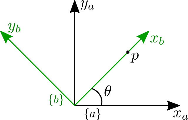
Figure 1: Schematic for the simple planar example
Let's rotate the components of the point \(p\) to be expressed in the \(\{b\}\) frame using a variety of rotation methods.
5.1.1 Rotation matrix
As an initial step, let's calculate the rotation matrix representing this rotation manually, and use that rotation matrix to transform the point. To describe the rotation from \(\{a\}\) to \(\{b\}\) as an element of \(SO(3)\), we need the components of the \(\{b\}\) basis vectors in the \(\{a\}\) frame. So we have the following:
\begin{align*} x_{ab} &= \left[\cos{\theta}\;\; \sin{\theta} \;\; 0 \right]\transpose \\ y_{ab} &= \left[-\sin{\theta}\;\; \cos{\theta} \;\; 0 \right]\transpose \\ z_{ab} &= \left[0 \;\; 0 \;\; 0 \right]\transpose \end{align*}Stacking these together as in the Rotation Matrix section we get
\begin{equation*} R_{ab} = \begin{bmatrix} 1/\sqrt{2} & -1/\sqrt{2} & 0 \\ 1/\sqrt{2} & 1/\sqrt{2} & 0 \\ 0 & 0 & 1 \end{bmatrix} \end{equation*}We can use the inverse of this matrix to transform \(p\) as follows:
\begin{equation*} p_b = R_{ba} p_a = R_{ab}\transpose p_a = \begin{bmatrix} 1/\sqrt{2} & -1/\sqrt{2} & 0 \\ 1/\sqrt{2} & 1/\sqrt{2} & 0 \\ 0 & 0 & 1 \end{bmatrix}\transpose \begin{bmatrix} 1/\sqrt{2} \\ 1/\sqrt{2} \\ 0 \end{bmatrix} = \begin{bmatrix} 1 \\ 0 \\ 0 \end{bmatrix} \end{equation*}From looking at Figure 1 this is exactly the result we expect. The only non-zero component of \(p\) in the \(\{b\}\) frame is the x component.
5.1.2 Axis and Angle to \(SO(3)\)
In this section we will show how an axis and angle can produce the same rotation matrix as in the previous section. Note that we haven't discussed these operations in this lecture, but most of the class is familiar with these operations from ME314 and ME449. If you are unfamiliar with the following operations, I recommend either the book A Mathematical Introduction to Robotic Manipulation or the 449 textbook Modern Robotics as good references. There are free PDFs of each of these books online.
The axis of rotation is \(\omega = [0 \;\;0 \;\;1]\transpose\) and the angle is \(\theta=\pi/4\). The skew-symmetric, cross product matrix for this axis is given by the hat operator
\begin{equation*} \hat{\omega} = \begin{bmatrix} 0 & -1 & 0 \\ 1 & 0 & 0 \\ 0 & 0 & 0 \end{bmatrix} \; \in so(3) \end{equation*}We can obtain the rotation matrix using the exponential map, which can be evaluated using Rodrigues' formula.
\begin{align*} R_{ab} &= e^{\hat{\omega}\theta} = I + \hat{\omega}\sin{\theta} + \hat{\omega}^2\left(1-\cos{\theta}\right) \\ &= \begin{bmatrix} 1 & 0 & 0 \\ 0 & 1 & 0 \\ 0 & 0 & 1 \end{bmatrix} + \begin{bmatrix} 0 & -1/\sqrt{2} & 0 \\ 1/\sqrt{2} & 0 & 0 \\ 0 & 0 & 0 \end{bmatrix} + \begin{bmatrix} -1 & 0 & 0 \\ 0 & -1 & 0 \\ 0 & 0 & 0 \end{bmatrix} \left( 1 - \frac{1}{\sqrt{2}} \right) \\ &= \begin{bmatrix} 1/\sqrt{2} & -1/\sqrt{2} & 0 \\ 1/\sqrt{2} & 1/\sqrt{2} & 0 \\ 0 & 0 & 1 \end{bmatrix} \end{align*}Clearly this is the same rotation matrix as in the previous section, and it will result in the same vector transform.
5.1.3 Quaternion Rotation
As mentioned in the previous section, the axis and angle are given by \(\omega = [0 \;\;0 \;\;1]\transpose\) and \(\theta=\pi/4\), respectively. Using Eq. \(\eqref{eq:quat_from_axis_angle}\) we can build our quaternion that represents this rotation as
\begin{align*} Q_{ab} &= \cos{\frac{\theta}{2}} + \left(w_x \mathbf{i} + w_y \mathbf{j} + w_z \mathbf{k} \right) \sin{\frac{\theta}{2}} \\ &= \cos{\frac{\pi}{8}} + 1 \mathbf{k} \sin{\frac{\pi}{8}} \\ &\approx 0.924 + 0.383 \mathbf{k} \end{align*}Now we "convert" our \(p\) vector into a quaternion form by appending a zero as the real part, and we use Eq. \(\eqref{eq:quat_rotation}\) to define the following rotation:
\begin{align*} P_b &= Q_{ab} \cdot P_a \cdot Q_{ab}^{-1} \\ &= \begin{bmatrix} 0.924 \\ 0 \\ 0 \\ 0.383 \end{bmatrix} \cdot \begin{bmatrix} 0 \\ 1/\sqrt{2} \\ 1/\sqrt{2} \\ 0 \end{bmatrix} \cdot \begin{bmatrix} 0.924 \\ 0 \\ 0 \\ -0.383 \end{bmatrix} \\ &= \begin{bmatrix} 0 \\ 1 \\ 0 \\ 0 \end{bmatrix} \\ \implies p_b &= \begin{bmatrix} 1 \\ 0 \\ 0 \end{bmatrix} \end{align*}5.2 Python Example
The following script contains several useful examples of converting between
representations, and for working with quaternions. There are also several
test functions that verify rotation matrices and quaternions obey the
properties that they are supposed to. These functions can be used for testing
the various conversion functions. The run_example_transforms() function
implements the example from the previous section, and the
perform_random_axis_and_angle_tests() function randomly generates rotation
axes and angles and then verifies the quaternion rotation function
(quat_transform) produces the same transformed result for a random vector
as a rotation matrix.
#!/usr/bin/env python
import numpy as np
import tf.transformations as tr
from math import pi
from random import gauss

ERRRED = '\033[91m'
ENDC = '\033[0m'

def matmult(*x):
  return reduce(np.dot, x)


def test_quat_props(Q, verbose=False):
    if verbose: print "Testing quaternion dimensions..."
    if len(np.ravel(Q)) is 4:
        if verbose: print "Passed"
    else:
        print ERRRED+"Failed"+ENDC
    if verbose: print "Testing quaternion norm...."
    if np.abs(np.linalg.norm(Q) - 1) < 1e-12:
        if verbose: print "Passed"
    else:
        print ERRRED+"Failed"+ENDC


def test_so3_props(R, verbose=False):
    R = np.array(R)
    if verbose: print "Testing SO(3) dimensions..."
    if R.shape[0] is 3 and R.shape[1] is 3:
        if verbose: print "Passed"
    else:
        print ERRRED+"Failed"+ENDC
    if verbose: print "Testing SO(3) inverse...."
    if np.max(matmult(R.transpose(),R)-np.eye(3)) < 1e-12:
        if verbose: print "Passed"
    else:
        print ERRRED+"Failed"+ENDC
    if verbose: print "Testing SO(3) determinate...."
    if np.linalg.det(R) - 1 < 1e-12:
        if verbose: print "Passed"
    else:
        print ERRRED+"Failed"+ENDC


def axis_angle_to_quat(w, th):
    return np.array(np.hstack((np.cos(th/2.0), np.array(w)*np.sin(th/2.0))))


def quat_to_axis_angle(Q):
    th = 2*np.arccos(Q[0])
    if np.abs(th) < 1e-12:
        w = np.zeros(3)
    else:
        w = Q[1:]/np.sin(th/2.0)
    return w, th


def hat(w):
    return np.array([
        [0, -w[2], w[1]],
        [w[2], 0, -w[0]],
        [-w[1], w[0], 0]])


def unhat(what):
    return np.array([-what[1,2], what[0,2], -what[0,1]])


def axis_angle_to_so3(w, th):
    return np.eye(3) + matmult(hat(w),np.sin(th)) + matmult(hat(w),hat(w))*(1-np.cos(th))


def so3_to_axis_angle(R):
    th = np.arccos((R.trace() - 1)/2)
    if (th <= 1e-12):
        th = 0.0
        w = 3*[1/np.sqrt(3)]
    else:
        w = 1/(2*np.sin(th))*np.array([R[2,1]-R[1,2], R[0,2]-R[2,0], R[1,0]-R[0,1]])
        if any(map(np.isinf, w)) or any(map(np.isnan, w)):
            th = 0.0
            w = 3*[1/np.sqrt(3)]
    return w, th


def quat_to_so3(Q):
    w, th = quat_to_axis_angle(Q)
    return axis_angle_to_so3(w, th)


def so3_to_quat(R):
    w,th = so3_to_axis_angle(R)
    return axis_angle_to_quat(w, th)


def quat_mult(Q,P):
    q0 = Q[0]
    p0 = P[0]
    q = Q[1:]
    p = P[1:]
    return np.hstack((q0*p0-np.dot(q,p), q0*p + p0*q + np.cross(q,p)))


def quat_conj(Q):
    return np.hstack((Q[0], -1*Q[1:]))


def quat_norm(Q):
    return np.linalg.norm(Q)


def quat_inv(Q):
    return quat_conj(Q)/quat_norm(Q)**2.0


def quat_transform(Q, p):
    pq = np.hstack((0,p))
    return quat_mult(quat_mult(Q,pq),quat_inv(Q))[1:]


def make_rand_unit_vector(dims):
    vec = [gauss(0, 1) for i in range(dims)]
    mag = sum(x**2 for x in vec) ** .5
    return [x/mag for x in vec]


def run_example_transforms():
    # create a vector in the "a" frame
    pa = [1/np.sqrt(2),1/np.sqrt(2),0]
    # create a rotation matrix from the "a" to the "b" frame (rotate pi/4 around z-axis):
    Rab = axis_angle_to_so3([0,0,1], pi/4.0)
    # get original vector expressed in the "b" frame:
    pb = matmult(Rab.T,pa)
    # create a quaternion for the same rotation:
    Qab = so3_to_quat(Rab)
    # transform using quaternion:
    pb_q = quat_transform(quat_inv(Qab), pa)
    # print results:
    print "Original Vector pa =",pa
    print "pb = Rba*pa =",pb
    print "Pbq = Qab*Pa*Qab^* =",pb_q
    print "Rab =",Rab
    print "Qab =",Qab
    return


def perform_random_axis_and_angle_tests():
    for i in range(100):
        # generate random axis:
        w = make_rand_unit_vector(3)
        pa = 20*np.random.random_sample((3,)) - 10
        for th in np.linspace(0, 2*pi, 30):
            Rab = axis_angle_to_so3(w, th)
            test_so3_props(Rab)
            pb = matmult(Rab.T, pa)
            Qab = axis_angle_to_quat(w, th)
            test_quat_props(Qab)
            pb_q = quat_transform(quat_inv(Qab), pa)
            if np.max(np.abs(pb-pb_q)) > 1e-12:
                print ERRRED+"[ERROR]"+ENDC
                print "pa = ",pa
                print "w = ",w
                print "th = ",th,"\r\n"
                break


if __name__ == '__main__':
    run_example_transforms()
    perform_random_axis_and_angle_tests()
6 Resources
Without a doubt, the most illustrative lessons I've seen on understanding the geometry of quaternions comes from the YouTube channel 3Blue1Brown. I'd highly recommend spending time studying the following lessons if you want to develop intuition about quaternions in general and their use in representing rotations.
- What are quaternions, and how do you visualize them? A story of four dimensions. This 30 minute video provides excellent animations to help you visualize the 4-dimensional space of quaternions and why the quaternion operations from these notes are defined they way they are.
- Visualizing quaternions: An explorable video series is the follow-on lesson to the previous video. This is a set of "explorable videos" where you can actually interact with the quaternion animations as the lesson is taught. I'd highly recommend spending an hour or two with this as a way to develop your own intuition about the geometry of unit quaternions as rotation representations.
Below is a list of other great resources
- Great YouTube video illustrating Gimbal lock
- This PDF of a talk called Understanding Quaternions given by from Jim Van Verth (a software engineer at Google) gives some great examples of how to use quaternions for representing rotations.
- The Charts on \(SO(3)\) Wikipedia page has discussions of several different parameterizations of \(SO(3)\) and the pros and cons of each. Note, this is a fairly mathematical page.
- The Wikipedia page on Euler Angles is a great reference on all of the different 3-parameter, elemental rotation parameterizations of \(SO(3)\).
- The Wikipedia page on Quaternions and spatial rotation is much more useful that the main Quaternion page for understanding how quaternions are used in geometry.
- The Wikipedia page on \(SO(3)\) provides a good description of this group.
- The book A Mathematical Introduction to Robotic Manipulation is a great resource on robot geometry in general. Chapter 2 contains concise descriptions of Euler angles and quaternions. The PDF is available online for free on the book's official page.
- The 449 textbook Modern Robotics is a great reference for all of these representations of rotation. In particular, Appendix B has excellent descriptions of Euler angles and quaternions.
- The tutorial paper Representing Attitude: Euler Angles, Unit Quaternions, and Rotation Vectors by James Diebel is a great reference for understanding the differences between various representations of orientation. There are excellent drawings, and many utility functions for converting between various representations. Note that all Euler angles in the paper are relative (intrinsic) rotations.
- As mentioned in the tf lecture, transformations.py is a Python module that is included with the tf package. It contains many functions for converting between different orientation representations.
