Particle Filters and Robot Localization
Table of Contents
1 Introduction
Filtering and estimation are a critical component of nearly every robotic system. Some people use the terms filter and estimator interchangeably, and others have a very specific definition of each. In this course, I will use them interchangeably. An estimator generally serves two purposes:
- Obtaining estimates of components of a system's state that are not directly measurable. These estimates are then typically used for controlling the system.
- Even for states that are measurable, one must deal with sensor noise. By combining a model of the system and a model of the sensor, we would like the estimator to provide estimates of the state that are more accurate than using either the model or the sensor alone.
In this topic, we will cover some basics of probability, then we will discuss a common filtering algorithm called a particle filter. Finally, we will spend a few minutes talking about how particle filters can be used for solving the so-called localization problem.
As a general note, the things discussed in this page are generally applicable to arbitrary systems, however, we are only discussing them in the context of the ROS navigation stack. Thus, we may sometimes treat aspects of the topics as if they are specific to 2D mobile robot navigation.
2 Basic Probability
Before we begin, we must have some basic definitions from probability theory.
2.1 Definitions
- Let's say that \(X\) is a discrete random variable. In other words, it is some variable that could take on a finite set of values (we don't know its exact value).
- \(x\) is a potential value of the random variable \(X\)
- Then we say that \(p(X=x)\) is the probability that \(X\) is \(x\). For example, let's take the classic example of a coin flip. Then \(X\) could either be \(heads\) or \(tails\). If we are interested in the probability that a random coin flip will produce one of the two values, we could write \(p(X=heads) = p(X=tails) = \frac{1}{2}\)
- For a discrete random variable \(X\), the following must hold \[ \sum\limits_x p(X=x) = 1 \qquad p(X=x) \ge 0 \,\forall\,x\]
- For a continuous random variable, we are usually interested in a probability density function (PDF). A PDF is a function that returns the relative likelihood that a sample from the continuous random variable will equal a given value. The PDF describes the "shape" of the distribution of \(X\).
- The following property must hold for a PDF \[ \int\limits_{-\infty}^{\infty} p(x) dx = 1\]
- An example PDF is that of a standard Gaussian or Normal distribution: \[ p(x) = \left( 2\pi \sigma^2\right) ^{-\frac{1}{2}} \exp{\left(-\frac{1}{2}\frac{(x-\mu)^2}{\sigma^2} \right)}\] where \(\mu\) is the mean of the distribution and \(\sigma^2\) is the variance.
- Joint distributions are distributions that depend on two different random variables i.e. \(p(x,y) = p(X=x \,\,\mathrm{and}\,\,Y=y)\).
- If \(X\) and \(Y\) are independent random variables, then \[ p(x,y) = p(x)p(y). \] For example, consider two coins where \(X\) is the result of flipping the first coin and \(Y\) is the result of flipping the second coin. The two processes are unrelated (the result of the second coin flip does not depend on the first). So \(X\) and \(Y\) are independent \[ p(X=heads,Y=heads) = p(heads,heads) = p(heads)p(heads) = \left(\Half\right) \left(\Half\right) = \frac{1}{4} \]
- Let's say we have to random variables \(X\) and \(Y\). Now let's say that
we happen to know the value of \(Y\) i.e. \(Y=y\). We want to know the
probability that \(X=x\) knowing that \(Y=y\). We write this as
\[ p(x \given y) = p\left(X=x \given Y=y\right). \]
- This type of probability is referred to as a conditional probability
- A conditional probability is defined as \[ p\left(x \given y\right) = \frac{p(x,y)}{p(y)}. \]
- If \(X\) and \(Y\) are independent then \[ p\left(x \given y\right) = \frac{p(x)p(y)}{p(y)} = p(x). \]
- The Theorem of Total Probability states that \[ p(x) = \int{p\left(x \given y\right) p(y) }\: Dy \]
- Bayes Rule says that if \(p(y)>0\) then \[ p(x \given y) = \frac{p(y \given x) p(x)}{p(y)} \]
- An expectation is defined as \[ E(X) = \int x\: p(x)\: dx \]
2.2 Bayes Theorem in Robotics
In this section, we provide some context to how the probability definitions listed above usually show up in the context of robotics. In a robotic system, the following are typical characteristics:
- \(x\) is the state or pose of a system (depending on whether we have a second order or a first order system). In the context of 2D mobile robot navigation, this is usually something like \(x = [x_r \; y_r \; \theta_r ]\transpose \)
- \(y\) is typically some sort of predicted sensor measurement given a particular state; i.e., this is what we would expect to measure if we were at some state \(x\)
- \(z\) is some sort of actual sensor measurement. If our sensor had no noise, we would expect \(y=z\) at the true state of the robot.
- Then the conditional probability \(p(x \given y)\) in words is the probability that the robot is at state \(x\) knowing that the measurement produced is value \(y\).
- When running filtering and estimation algorithms, the following terms are
often used:
- \(p(x)\) - prior probability distribution: Here, the word prior is used to indicate that we have not yet incorporated a measurement. This is analogous to a prediction of the robot's state uncertainty.
- \(z\) - data: This is the data that comes from a sensor.
- \(p(x \given z)\) - posterior probability distribution: This is the uncertainty in the robot's state after incorporating a measurement.
2.2.1 State Transition Probability
The state transition probability is the probability of a particular state \(x\) at a particular time \(t\) given all past states \(x_{0:t-1}\), measurements \(z_{1:t-1}\), and controls \(u_{1:t}\). I.e., \[ p\left(x_t \given x_{0:t-1}, z_{1:t-1}, u_{1:t}\right) \] Note that in the above, the measurement at time \(t\) has not been taken into account.
In robotics, we typically deal only with something referred to as a Markov chain. A Markov chain is nothing more than a discrete set of random events where the future state of the system is defined completely by the current state. In other words, knowledge of past states contributes nothing to the future knowledge. In robotics, this is equivalent to saying that knowing the current probability distribution of the system and the current control is sufficient for predicting the distribution at the next sequence. In this case, the state transition probability reduces to \[ p\left(x_t \given x_{t-1}, u_{t}\right) \] This is the situation we will exclusively consider.
2.2.2 Measurement Probability
Typically, our robotic system has some sort of function that would allow us to map a state into a predicted measurement. In other words, if we are at some state \(x\) what is the measurement from our sensor that we should expect to see \(y\). For example, imagine a mobile robot navigating in the plane that has a range sensor capable of measuring the distance to the \(x\)-axis. Then our measurement model (or output model) would be something like \[ y = g(x) = \left[0 \;1 \;0\right] \begin{bmatrix} x_r \\ y_r \\ \theta_r \end{bmatrix} \]
Now, typically we will know that our sensors aren't perfect, and we will have some sort of PDF representing our uncertainty in the measurements received. Given this PDF, the term that we will be interested in evaluating is the probability that we would measure some particular measurement \(z\) at time \(t\) if we are at a particular state \(x\). In other words, we need to be able to evaluate a measurement probability given by \(p(z_t \given x_t)\).
2.2.3 Belief Distributions
The term belief distribution often shows up in robotics. This is defined as the robot's internal knowledge about the state of the environment. It is nothing more than a posterior probability at a particular time given all available data. As an equation, the belief of state \(x\) at time \(t\) is given by \[ bel(x_t) = p\left(x_t \given z_{1:t},u_{1:t}\right) \]
A prediction or proposal belief distribution is the predicted belief before incorporating a measurement \[ \overline{bel}(x_t) = p(x_t \given z_{1:t-1}, u_{1:t}) \]
3 Particle Filters
In a particle filter, we are going to represent our belief distribution \(bel(x_t)\) using a finite collection of parameters called particles. We don't need a mathematical expression for the PDF representing our belief. Rather, we assume that this collection of particles is a set of random samples drawn from this PDF. In this way, the set of particles represents an approximation of the belief distribution. Particle filters are one of the most general filters because we don't require any special parameterizations of any distributions. This is especially convenient in robotics because it allows us to pass our distributions through nonlinear transformations without requiring any special mathematical machinery. Other filters (such as histogram filters or Kalman filters) require us to parameterize our uncertainty distributions, and then the filter will predict the evolution of these parameters. This is problematic because we are then often restricted to simple distributions and simple system dynamics.
In the particle filter, we will call denote our sampling of our belief using \(M\) particles as \[ \mathcal{X}_t \equiv x_t^1, x_t^2, \ldots, x_t^M \]
We will recursively construct the belief at time \(t\) from the collection of particles at the previous time. In other words, \(bel(x_t)\) will be constructed from \(bel(x_{t-1})\).
3.1 Algorithm
The algorithm for the particle filter is given below:
particle_filter\((\mathcal{X}_{t-1}, u_t, z_t)\):
\(\overline{\mathcal{X}}_t = \mathcal{X}_t = W_t = \mathrm{zeros}\) # initialize empty arrays
for \(m=1\) to \(M\) do:
sample \(x_t^m \sim p(x_t \given u_t, x_{t-1}^m)\) # get particle \(m\) by drawing a random sample from state transition distribution
\(w_t^m = p(z_t \given x_t^m)\) # calculate "importance factor" or "weight" for particle \(m\)
\(\overline{\mathcal{X}}_t[m], \, W_t[m] = x_t^m, \, w_t^m\) # store weights and particles
endfor
for \(m=1\) to \(M\) do:
draw \(i\) w/probability \(\propto w_t^i\) # choose a random particle index \(i\); higher weight \(\implies\) higher probability
add \(x_t^i\) to \(\mathcal{X}_t\) # store random particle in new particle collection
endfor
return \(\mathcal{X}_t\)
So, in order to run this algorithm, there are a few things that we need to know how to do.
- We need to be able to sample from the state transition model. So we are going to need some function that will return a random sample from \(p(x_t \given u_t, x_{t-1}^m)\)
- We need a measurement model \(p(z_t \given x_t^m)\)
- In the second for-loop, we re-sample our particle set with replacement. So we need some way to "resample" our particle set with probabilities proportional to the importance factors.
These three items will be discussed in the following sections.
3.2 Resampling
The second for-loop in the particle filter algorithm of the previous section is the key to the particle filter's functionality. This resampling process is how measurements are incorporated. Basically, in the first for-loop, we calculate a "weight", also called an "importance factor" for each particle. Given a measurement model and an actual measurement taken at time \(t\), \(z_t\), we evaluate the probability of reading that measurement for each particle (\(p(z_t \given x_t^m)\)). We assume that the actual measurement reading obeys some noise model. So if we consider a particle that is very near the true state of our robot the probability that we would have received the particular sensor reading that we did receive should be high. In other words, if we actually put the robot at the state of the particle, and took a sensor reading we would have high probability that the sensor reading is close to the one that we did receive. If we consider a particle that is far from the true state, the probability that we would have received the particular sensor reading if the robot were at that state is low.
When we resample, we are creating a new collection of particles (same number of particles) that now represent a sampling of the posterior distribution (a distribution that has the information from the new measurement incorporated). This is done by giving higher probability of resampling a particular particle to particles that have high weight. In this way, the resampled collection of particles will have shifted towards the measurement. Later on, in the examples section, we will provide example Python code that illustrates this resampling procedure.
3.3 Measurement Models
There are many different ways to represent \(p(z_t \given x_t)\). The "correct" way depends strongly on the particular system and the sensor being used. In the situation where you are considering a robot navigating around in a 2D world with something like a laser scanner, you could have the following categories of noise:
- Regular sensor noise: E.g. regular Gaussian noise introduced by the characteristics of the sensor.
- Unexpected objects: This is what happens when the sensor measures objects that weren't expected to be there. For example, let's say you have a map of the environment that your robot is expecting to see, but there is a person walking around that the map does not account for.
- Failures: This is the situation where your sensor fails to return a reading when it should.
- Random measurements: Situations where the sensor returns a false reading that suggests there is an object where there isn't one.
You could come up with separate noise models for each of these categories, and then combine them all together to build a single noise model. This is exactly what the ROS package AMCL does. Each of these noise models have very different characteristics, and typically, there are already some basic models to describe these characteristics. Given a particular sensor, it is then up to you to figure out how to fit the parameters of each of these models to your particular sensor.
As a simple example, let's look at the noise model for the first category; regular sensor noise. We model this noise with a simple Gaussian centered at the true measurement value and with a variance \(sigma^2\). Ideally, this variance corresponds to the true variance that you would expect from your sensor. Now, let's assume that at time \(t\) the true value of our system is \(z^*_t\). Then, we would expect our actual measurement taken at time \(t\), \(z_t\) to be sampled from a Gaussian \(\mathcal{N}(z_t^*,\sigma^2)\). We need a way, for a given particle \(x_t^m\) to evaluate \(p(z_t \given x_t)\). All we have to do with this measurement model is assume that our distribution is centered around our particle, and then the PDF for a Gaussian allows us to evaluate
\[ p(z_t \given x_t) = \frac{1}{\sqrt{2\pi \sigma^2}}\exp{\left[-\Half \frac{\left(z_t - g(x_t^m)\right)^2}{\sigma^2} \right]} \]
where \(z=g(x)\) is a nonlinear mapping from state to expected measurement (this is often called an observation model or output model). In this equation, if the particle is near \(z^*_t\), then it is likely that the above probability will be high.
3.4 State Transition Model for a Kinematic Car
In order to implement a particle filter, we must be able to sample from \(p(x_t \given u_t, x_{t-1}^m)\). For an arbitrary system, there are many ways to come up with an algorithm that allows this sampling. A common technique is to assume that all noise is introduced in the controls. In other words you assume that all stochastic behavior in your system comes from your stochastic behavior in your controls. You then must figure out how this noise maps through your system dynamics. In this section, we will come up with this model for a kinematic car.
We are going to assume that over a time interval \((t-1,t]\) the robot maintains a constant angular and translational velocity \((v,\omega)\). Then we know at some instant in this time interval the robot is traveling in a perfect circle of radius \[ r = \left \lvert \frac{v}{\omega} \right \rvert \] In the above if \(\omega=0\), the robot is traveling in a straight line, and the radius is infinity.
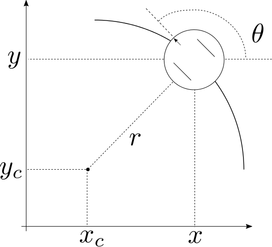
Figure 1: Geometry of the kinematic car.
If we let the state at \(t-1\) be given by \(x_{t-1} = [x \; y \; \theta]\transpose\), then we can calculate the location of the center of the circle that the robot is traveling on as
\begin{align*} x_c &= x - \frac{v}{\omega}\sin{\theta} \\ y_c &= y + \frac{v}{\omega}\cos{\theta} \end{align*}Now we are interested in where the robot ends up after \(\Delta t\) seconds. This can be calculated from simple geometry as
\begin{align*} x_t = \begin{bmatrix} x^\prime \\ y^\prime \\ \theta^\prime \end{bmatrix} &= \begin{bmatrix} x_c + \tfrac{v}{\omega}\sin{\left(\theta + \omega \Delta t \right)} \\ y_c - \tfrac{v}{\omega}\cos{\left(\theta + \omega \Delta t \right)} \\ \theta + \omega \Delta t \end{bmatrix} \\ &= \begin{bmatrix} x \\ y \\ \theta \end{bmatrix} + \begin{bmatrix} -\tfrac{v}{\omega}\sin{\theta} + \tfrac{v}{\omega}\sin{\left(\theta + \omega \Delta t \right)} \\ \tfrac{v}{\omega}\cos{\theta} - \tfrac{v}{\omega}\cos{\left(\theta + \omega \Delta t \right)} \\ \omega \Delta t \end{bmatrix} \end{align*}If we now assume that the actual velocities are not exactly the specified \(v\) and \(\omega\), we can begin to model this as a noisy system. Assume that the true velocities are given by
\begin{equation*} \begin{bmatrix} \hat{v} \\ \hat{\omega} \end{bmatrix} = \begin{bmatrix} v \\ \omega \end{bmatrix} + \begin{bmatrix} \xi_1 \\ \xi_2 \end{bmatrix} \end{equation*}where the \(\xi_i\) are random samples drawn from some distribution. Now if we substitute these velocities into the transition equation above, we have a simple technique for drawing samples from a random state evolution. However, this is not yet perfect because we are still assuming perfectly circular motion throughout our \(\Delta t\). In reality, we should be able to arrive at any \([x^\prime \; y^\prime \; \theta^\prime]\transpose\), but this model restricts how noise evolves more than we would like. A simple solution is to add a third random variable that is simply a rotation at the end of the motion. So the new angle is given by
\[ \theta^\prime = \theta + \hat{\omega} \Delta t + \hat{\gamma} \Delta t . \]
In many situations, it is also desirable to assume that the levels of noise are proportional to velocity. Intuitively, this makes sense. If the robot has zero velocity, we shouldn't expect it to move very much during a timestep. If a robot is driving fast, we expect that our models of its kinematics become less accurate; at high speeds we may be more susceptible to phenomena such as wheel slippage. So the model for the random inputs is given by
\begin{equation*} \begin{bmatrix} \hat{v} \\ \hat{\omega} \\ \hat{\gamma} \end{bmatrix} = \begin{bmatrix} v \\ \omega \\ 0 \end{bmatrix} + \begin{bmatrix} \text{sample}\left(\alpha_1 v^2 + \alpha_2 \omega^2\right) \\ \text{sample}\left(\alpha_3 v^2 + \alpha_4 \omega^2\right) \\ \text{sample}\left(\alpha_5 v^2 + \alpha_6 \omega^2\right) \end{bmatrix} \end{equation*}The \(\text{sample}\) function draws a single number from an arbitrary distribution with variance given by the argument i.e. large values of \(\alpha_i\) result in large values of noise. This is exactly the state transition model used by AMCL. An example implementation of this will be given below.
4 Issues With Particle Filters
In this section, we will present several common issues and concerns related to implementing particle filters.
- Computational Complexity
- With particle filters, computational complexity is a big concern because all operations must be carried out for each particle. So it is important to use the "right" number of particles. If you have too many particles, you are wasting computation, and too few particles may result in inaccurate representations of the distributions. Note that there are some algorithms for automatically adjusting the number of particles on the fly. Additionally note that particle filter algorithms are often easily parallelized; running in parallel can save great computational expense with minimal programming effort.
- Resampling Uniqueness
- When we resample, we are reducing the count of unique particles. In the worst-case scenario, if the robot is stationary and we run the particle filter long enough, we may reduce the number of unique particles all of the way down to one. In this case, the estimates of the posterior distribution are completely useless. There are multiple strategies that people employ to counteract this issue. For example, one heuristic would be to add an arbitrary rule that stops resampling when velocities are below a threshold. Another technique would be to inject random particles after resampling, or even to add some stochastic behavior to the resampling process (occasionally resample low-weight particles).
- Particle Deprivation
- A related issue is called particle deprivation. Particle deprivation is when there are not enough particles in the vicinity of the true state, and the resampling procedure ends up drastically reducing the number of unique particles. This may be caused by having too few particles in your state space.
- Density Extraction
- After completing a step of the particle filtering
algorithm, the particles represent a sampling of the posterior
distribution. However, in many situations, it may be desirable to have an
analytical PDF that represents this distribution (rather than just a
sampling). So we want to transform from the collection of particles to
the PDF function that describes the distribution the particles were
sampled from. There are a variety of techniques for this procedure. Some
possible techniques to read about are:
- Gaussian approximations
- K-means clustering
- Density trees
- Kernel density estimation.
5 Examples
In this section, we will provide several code samples that demonstrate the procedures from above.
5.1 Uniform Resampling
The following script imagines 1-D state values for three particles, and three corresponding weights. It then shows several different algorithms for performing the resampling process biased by the weights.
import numpy as np
from collections import Counter

# generate a random set of 1D "particles"
particles = [1.2, 2.6, 1.7]
# generate a pre-normalized set of weights for each particle:
weights = [0.3, 0.1, 0.6]
# so there is a 30% chance that we will resample particle 0, a 10% chance we
# will resample particle 1, and a 60% chance we will resample particle 2


# now let's write a simple resampling function:
def resample_simple(particles, weights, size=None):
    if size is None:
        size = len(particles)
    # create empty array for storing particles:
    new_particles = np.zeros(size)
    # ensure weights are normalized:
    w_norm = np.array(weights)/np.sum(weights)
    for m in range(size):
        # generate a random number in [0,1):
        u = np.random.random_sample()
        # iterate to figure out which particle to resample:
        wmin = 0.0
        for i,w in enumerate(w_norm):
            # in below 'if' statement, the probability that u is contained
            # inside of an interval of 'w' width exactly corresponds to the
            # probability of resampling particle i
            if u >= wmin and u < wmin+w:
                new_particles[m] = particles[i]
                break
            wmin += w
    return new_particles


# let's write a new version of the last function using a couple of fancy numpy
# functions:
def resample_fancy(particles, weights, size=None):
    if size is None:
        size = len(particles)
    ranges = np.cumsum(weights/np.sum(weights))
    return np.array(particles)[np.digitize(np.random.random_sample(size), ranges)]


def main():
    # Let's draw samples using each of these algorithms, and print the results. Note
    # that as the number of particles goes up, the accuracy of the resampling
    # algorithms increases.
    new_simple_default = resample_simple(particles, weights)
    new_fancy_default = resample_fancy(particles, weights)

    new_simple_20particles = resample_simple(particles, weights, size=20)
    new_fancy_20particles = resample_fancy(particles, weights, size=20)

    new_simple_50000particles = resample_simple(particles, weights, size=50000)
    new_fancy_50000particles = resample_fancy(particles, weights, size=50000)

    def print_analysis(name, weights, old_particles, new_particles):
        c = Counter(new_particles)
        print "=================================================="
        print name
        for w,p in zip(weights,old_particles):
            print "{0:2.2f}% of particles are {1:2.2f} (expected {2:2.2f}%)".format(100*c[p]/float(len(new_particles)), float(p), 100*w)
        print "=================================================="
        print "\r\n",
        return

    print_analysis("Simple default size", weights, particles, new_simple_default)
    print_analysis("Fancy default size", weights, particles, new_fancy_default)
    print_analysis("Simple size=20", weights, particles, new_simple_20particles)
    print_analysis("Fancy size=20", weights, particles, new_fancy_20particles)
    print_analysis("Simple size=50000", weights, particles, new_simple_50000particles)
    print_analysis("Fancy size=50000", weights, particles, new_fancy_50000particles)

if __name__ == '__main__':
    main()
5.2 Importance Resampling
The following script shows how we can calculate weights for a set of
particles, and resample based on these weights to represent a different
distribution. In the example, we have a set of particles called
source_samples drawn from a PDF given by g(x). We are going to calculate
weights for each of these particles based on a target distribution f(x).
When we resample based on these weights, the new set of particles represents
a sampling of the target distribution. Note that this example uses the
resample_fancy function from the previous example.
import numpy as np
import matplotlib.pyplot as mp
from uniform_resample import resample_fancy

"""
This script illustrates how importance resampling can be used to take a
collection of particles sampled from a source distribution and represent a
different target distribution.
"""

SIZE = 5000

##################
# DISTRIBUTIONS: #
##################
# Weibull distribution w/ \lambda=1, a=1.5 will form our source distribution
# https://en.wikipedia.org/wiki/Weibull_distribution
a = 1.5
source_samples = np.random.weibull(a, size=SIZE)
def g(x):
    return a*x**(a-1)*np.exp(-x**a)

# Normal distribution with \mu=0.5, and \sigma=0.2 will form our target
# distribution
mu = 1.5
sigma = 0.2
target_samples = np.random.normal(mu, sigma, size=SIZE)
def f(x):
    return 1/(sigma*np.sqrt(2*np.pi))*np.exp(-(x-mu)**2.0/(2*sigma**2.0))

###########################
# PLOTTING AND RESAMPLING #
###########################
# plot both the target and the source distribution:
n_source, bins_source, patches_source = mp.hist(source_samples, 100, normed=1, facecolor='green', alpha=0.25)
n_target, bins_target, patches_target = mp.hist(target_samples, 50, normed=1, facecolor='blue', alpha=0.25)

# add best fit PDFs for both distributions:
x_source = np.linspace(np.min(source_samples), np.max(source_samples), 1000)
y_source = g(x_source)
mp.plot(x_source, y_source, 'g--', lw=2)

x_target = np.linspace(np.min(target_samples), np.max(target_samples), 1000)
y_target = f(x_target)
mp.plot(x_target, y_target, 'b--', lw=2)

# now, let's calculate the weights for each sample in the source distribution
# using the target PDF, and then, let's resample according to those weights
weights = np.array([f(x)/g(x) for x in source_samples])
new_samples = resample_fancy(source_samples, weights)
n_new, bins_new, patches_new = mp.hist(new_samples, 100, normed=1, facecolor='red', alpha=0.25)

mp.show()
5.3 Sample Measurement Model
This example sets a 1D robot at a known location x=1. It then generates a
fake measurement by drawing a single sample from a distribution centered at
1. Based on this measurement, we calculate weights for each particle, and
resample based on these weights. Note that as the iterations continue, this
particle filter will eventually suffer from particle uniqueness issues.
import numpy as np
import matplotlib.pyplot as mp
from uniform_resample import resample_fancy
from itertools import cycle

"""
In this example, let's assume that we have a 1-D robot located exactly at
x=1. Let's also assume that the robot has a range sensor that measures the
distance to the origin. We will assume that noise in our sensor can be
accurately described using a Gaussian.

This script will then do the following:
  1) Draw a random collection of particles that represents \bar{bel}(x_{t-1}).
  2) Generate an artificial "measurement" using a noisy measurement model
  3) Calculate weight of each particle
  4) Resample
  5) Iterate
"""

# define global constants:
NUM_PARTICLES = 1000
NUM_ITERATIONS = 5
DIVISOR = 1
NUM_SAVES = NUM_ITERATIONS/DIVISOR
X_GROUND_TRUTH = 1.0

# define variables for generating initial particle distribution, and sample
# particles:
mu_initial = X_GROUND_TRUTH + 0.2
sigma_initial = 0.2
Xt = np.random.normal(mu_initial, sigma_initial, size=NUM_PARTICLES)

# define parameters for measurement model and write function for evaluating
# p(z_t|x_t):
mu_measurement = X_GROUND_TRUTH
sigma_measurement = 0.05
def generate_measurement():
    return np.random.normal(mu_measurement, sigma_measurement)

def prob_zt_given_xt(zt, xt):
    return 1/(sigma_measurement*np.sqrt(2*np.pi))*np.exp(-(zt-xt)**2.0/(2*sigma_measurement**2.0))


# iteratively update particle collections using simple particle filter
# algorithm:
X_data = np.zeros((NUM_SAVES+1, NUM_PARTICLES))
Z_data = np.zeros(NUM_SAVES+1)
X_data[0] = Xt
Z_data[0] = X_GROUND_TRUTH
save_count = 0
for i in range(NUM_ITERATIONS):
    # generate a random measurement:
    zt = generate_measurement()
    # now calculate the weights for every particle:
    weights = np.array([prob_zt_given_xt(zt, x) for x in Xt])
    # resample according to weight probability:
    Xt = resample_fancy(Xt, weights)
    if (i+1)%DIVISOR == 0:
        # store data for plotting:
        X_data[save_count+1] = Xt
        Z_data[save_count+1] = zt
        save_count += 1

# now let's plot the data:
col_gen = cycle('bgrcmk')

def plot_step(ax, zt, Xt, color):
    n, bins, patches = ax.hist(Xt, 20, normed=True, facecolor=color, alpha=0.35)
    ax.plot([zt,zt],[0,max(n)],color=color,lw=2)
    ax.plot([X_GROUND_TRUTH,X_GROUND_TRUTH],[0,max(n)],'--',color='black',lw=2)
    ax.set_yticks([0,int(max(n))])
    def f(x):
        return 1/(sigma_measurement*np.sqrt(2*np.pi))*np.exp(-(x-mu_measurement)**2.0/(2*sigma_measurement**2.0))
    x_target = np.linspace(X_GROUND_TRUTH-0.5, X_GROUND_TRUTH+0.5, 1000)
    y_target = f(x_target)
    ax.plot(x_target, y_target*max(n)/20.0, '--', lw=1, color=color)
    return

f, axarr = mp.subplots(NUM_SAVES, sharex=True)
for z,x,ax in zip(Z_data, X_data, axarr):
    plot_step(ax,z,x,col_gen.next())

mp.show()
5.4 Sample Kinematic Car Model
This example uses two different implementations of a function for sampling
the kinematic car motion model. The sample_motion_model_velocity function
takes in a single state, a single control, and a timestep. It generates a new
random set of controls, and then uses the motion model to integrate these
noisy controls forward. The sample_motion_model_onestep function does the
same thing except it operates on an entire set of particles at once. This
implementation is much more computationally efficient.
import numpy as np
import matplotlib.pyplot as mp
import matplotlib.patches as patches
from itertools import cycle

"""
In this example, we illustrate how the motion model derived in class (with
noisy inputs) can be used to sample from p(x_t | x_{t-1},u_t)
"""

####################
# GLOBAL CONSTANTS #
####################
NUM_PARTICLES = 500
DT = 0.01
NUM_ITERATIONS = 100
DIVISOR = 20
# NUM_SAVES will define how many sets of particles we want to save and plot
# (NUM_ITERATIONS would likely be too many):
NUM_SAVES = NUM_ITERATIONS/DIVISOR
# Set initial conditions and control vector:
X0 = np.array([0,0,0])
unom = np.array([1,1])

####################
# NOISE PARAMETERS #
####################
a1 = 0.01
a2 = 0.01
a3 = 10
a4 = 0.01
a5 = 0.01
a6 = 0.01


# A simple function that takes in a single state, input, and timestep, and returns
# a sample from the noisy state transition model:
def sample_motion_model_velocity(x, u, dt):
    def sample(variance):
        return np.random.normal(0.0, np.sqrt(variance))
    v = u[0]
    w = u[1]
    vhat = v + sample(a1*v**2. + a2*w**2.)
    what = w + sample(a3*v**2. + a4*w**2.)
    ghat = sample(a5*v**2. + a6*w**2.)
    xp = x[0] - (vhat/what)*np.sin(x[2]) + (vhat/what)*np.sin(x[2] + what*dt)
    yp = x[1] + (vhat/what)*np.cos(x[2]) - (vhat/what)*np.cos(x[2] + what*dt)
    thp = x[2] + what*dt + ghat*dt
    return np.array([xp,yp,thp])


# A slightly modified version of the previous function where we take in an
# entire collection of particles, a single control, and a timestep. The function
# returns a new particle collection representing a sample from the state
# transition model for each of the original particles:
def sample_motion_model_onestep(X, u, dt):
    def sample(variance):
        return np.random.normal(0.0, np.sqrt(variance), size=len(X))
    v = u[0]
    w = u[1]
    vhat = v + sample(a1*v**2. + a2*w**2.)
    what = w + sample(a3*v**2. + a4*w**2.)
    ghat = sample(a5*v**2. + a6*w**2.)
    Xout = np.zeros(X.shape)
    Xout[:,0] = X[:,0] - (vhat/what)*np.sin(X[:,2]) + (vhat/what)*np.sin(X[:,2] + what*dt)
    Xout[:,1] = X[:,1] + (vhat/what)*np.cos(X[:,2]) - (vhat/what)*np.cos(X[:,2] + what*dt)
    Xout[:,2] = X[:,2] + what*dt + ghat*dt
    return Xout


# initialize a particle collection, a time vector, and an array for storing data:
Xt = np.zeros((NUM_PARTICLES, 3))
Xt[:,:] = X0
X_data = np.zeros((NUM_SAVES+1, NUM_PARTICLES, 3))
X_data[0] = Xt

# now we can run our simulation loop:
save_count = 0
for i in range(NUM_ITERATIONS):
    # SLOW:
    # Xt = np.array([sample_motion_model_velocity(x,unom,DT) for x in Xt])
    # FAST:
    Xt = sample_motion_model_onestep(Xt, unom, DT)
    if (i+1)%DIVISOR == 0:
        X_data[save_count+1] = Xt
        save_count += 1

def plot_cloud(ax, Xt, color, arrows=True):
    if arrows:
        def build_arrow(state, color):
            length = 1.5e-2
            return patches.Arrow(state[0], state[1], np.cos(state[2])*length, np.sin(state[2])*length, alpha=0.5, color=color, width=1e-2)
        for x in Xt:
            ar = build_arrow(x, color)
            ax.add_patch(ar)
    else:
        ax.plot(Xt[:,0], Xt[:,1], 'o', markersize=1.25, mec=color, mfc=color, alpha=0.7)
    return

col_gen = cycle('bgrcmk')
ax = mp.gca()
for x in X_data:
    plot_cloud(ax, x, col_gen.next(), arrows=False)
ax.axis('equal')
mp.show()
6 Particle Filters for Localization
6.1 Localization introduction
Localization is nothing more than determining where a robot is relative to some sort of known map using sensor data (typically a sensor on-board the robot). This is different than estimation because you typically cannot measure the robot's pose directly.
- Global/Local
- Sometimes the initial pose of the robot is known, and sometimes it is not. If the initial pose is known this is referred to as local localization. If the initial pose is not know, this is global localization.
- Dynamic Obstacles
- The robot's situation may involve some dynamic obstacles. For example, imagine you have a robot navigating in a static, unchanging environment (e.g. a school), but there are also people walking around (dynamic obstacles). Typically if there are dynamic obstacles, you either add the dynamic obstacles into the state of your system (you are estimating the pose of your robot and all dynamic obstacles), or you filter out the dynamic obstacles somehow.
- SLAM
- If the map is not known ahead of time, this is referred to as Simultaneous Localization and Mapping (SLAM).
- Active/Passive
- Sometimes localization is a passive process where the robot is attempting to accomplish some designated task, and localization is simply a necessary part of carrying out the bigger goal. Other times, the localization (and possibly mapping) is the ultimate goal of the robot. In this situation, the robot can guide its motions to optimize the effectiveness of the localization. For example, it can specifically search for distinguishing features that could help with localization.
- Multi-Robot Localization
- Sometimes you have more than one robot navigating in a map. You could have each robot localize independently. In this situation, each robot would just treat the other robots as dynamic obstacles. Alternatively, if the robots can communicate with each other, they can share their localization results. When working together, the team of robots can often be more effective at localizing.
6.2 Monte-Carlo Localization
The basic algorithm is referred to as Monte-Carlo Localization (MCL). They are really just particle filters slightly adapted to solve the localization problem. Note that many other estimation algorithms may be adapted to solve the localization problem. For example, other algorithms for localization are grid localization techniques, Markov localization, and multi-hypothesis tracking.
For the simplest case of MCL the map is nothing more than a set of features and their known locations. For example, the features could be the locations of several known tags, fiducials, or colored marks. Then all we really need to do is modify our measurement model to include details about the features. We then run a for-loop where we evaluate a probability for each of the possible features. The new version of the measurement model would be something like
\[ p(f_t^i \given c_t^i, m, x_t) \] where
- \(f_t^i\) is what was measured for feature \(i\). Commonly, this is the range and bearing to the detected feature, but it may also include details such as the color of the feature that was measured.
- \(c_t^i\) is the true identifier for the feature. When we run the for-loop we are iterating through each of the features to try and find the feature with the highest probability.
- \(m\) is the map. This is typically the locations (and any other information) of all of the features in the environment.
- \(x_t\) is the current state of the robot. Given this state and the map, for a given feature, we can determine what we should expect to measure. If there is high probability of measuring \(f_t\) for this feature, then particles at this state will get high weight.
The "features" that are used in MCL are often just rows of raw sensor readings (as would be expected from a 1D laser scanner). Then the map is just a bunch of points sampled along the obstacles that we expect to see. This is roughly how AMCL works.
6.3 Issues with MCL
- Complexity
- One huge issue is computational complexity. We are now considering many particles and many features, and the computational complexity is growing exponentially. Great care must be taken to ensure computationally feasible implementations.
- False Hypothesis
- Occasionally, a given particle may show have a high
weight for the wrong particle. In this case, we may end up resampling
particles that are not in the region of the true state of the robot.
This can quickly lead to serious particle deprivation. A related
situation is called the kidnapped robot problem imagine your robot is
localized, and then randomly someone picks up the robot and "teleports"
it to a new location in the map. For a given localization algorithm, one
hopes that they algorithm will automatically re-localize to the new
location. There are several ways to solve this problem:
- If you use huge numbers of particles, the likelihood of this situation is reduced. Of course, this results in high computational complexity.
- Sometimes this problem is avoided by randomly injecting particles into the state space. If you have localized onto false features, these random particles will hopefully help the system re-localize onto the correct feature.
- The above solutions work well, but they are difficult to tune. An alternative is an algorithm that will automatically adapt the numbers of particles and the random noise injection as the algorithm is running. This is what the "A" in the AMCL package stands for. Essentially, this algorithm adjust the number of particles and the random noise injections based on statistics of the probability distributions.
